Polarization Multi-Image Synthesis with Birefringent Metasurfaces

Motivation

Computational imaging systems are designed to solve inverse problems. For example: given a measured 2D projection of a 3D scene (i.e. an image captured on a phone), we may seek to produce a depth-map specifying the distance of each object. We may alternatively want to determine the phase of the light emitted from the scene or sample the images formed from light-rays of particular angles. All of these properties (depth of origin, phase, angular distribution) exist for light but are not easily identified using conventional cameras. Instead, to efficiently extract more information from a scene while using standard hardware, digital post-processing is often used. Through computing on the image(s) that we do have from our camera, the missing pieces of information can be "reconstructed" by leveraging our understanding of the measurement process and by making assumptions about what the answer is likely to be (this is called asserting priors).

In the long history of imaging research focused on solving these inverse problems, there is a fundamental principle which has always remained true: Extracting information is easier when computing on multiple images instead of just one! Notably, I am referring to multiple images of the same scene that are each captured from a different perspective or through a different set of optical components. Each image thus provides us with new information and enables us to either obtain the exact solution to the inverse problem without ambiguity or to do so while relying less on our priors. This fact serves as a key motiation for this work. To give a more concrete example of this principle, let us consider some methods to estimate depth maps (a distance value for each pixel in a 2D image of a scene). For those who are more familiar with computational imaging methods and research, feel free to skip ahead. Note that this project is not about depth-sensing but is instead focused on the design and optimization of a system that can capture multiple images of a scene in a single exposure.

When capturing an image of a scene, we measure a 2D projection of the intensity emitted or reflected from objects. Naturally, we cannot tell the exact depth that each object was at the time of the capture just by looking at our measured image but we have some guesses. For example, we can leverage the fact that real lenses produce sharp, in-focus images only for objects located at a particular depth (dependent on the lens's focal distance). 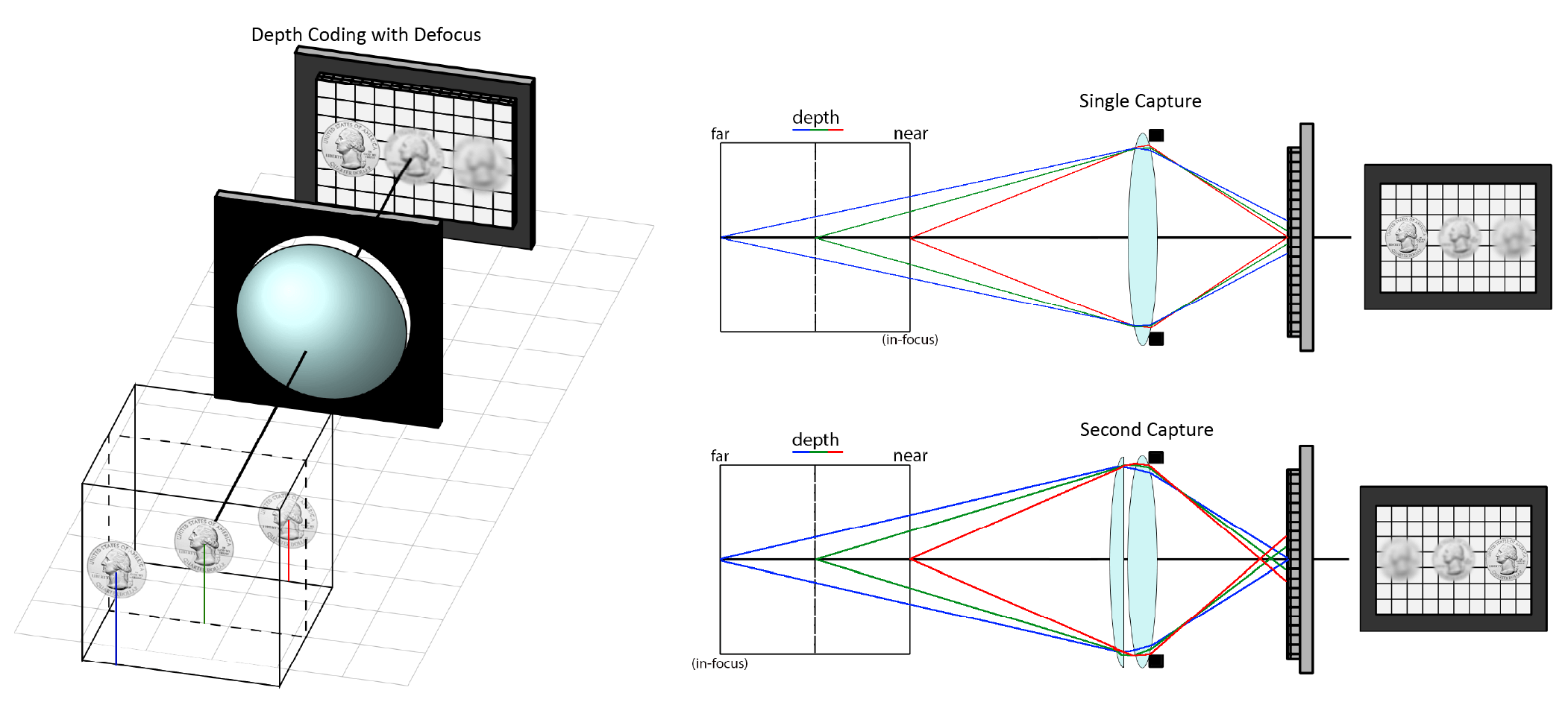This effect is subtle for images captured on your phone since the diameter of the lens is small and produces an extended "depth-of-field", but it is infact very noticible with larger cameras. As depicted in the diagram below, a single capture of a scene containing three quarters at different depths can produce an image where only one of the three coins is in focus while the other two have some gaussian blur. Depth is thus "coded" in the amount of blur and using this fact, it is possible to produce, through suitable computation, a depth-map of the scene from at minimum a single capture (top right).

It should be noted, however, that computing a depth-map of suitable accuracy and confidence from a single image alone is quite challenging! Using only the captured image that we have, we must first use our own reasoning and prior knowledge to recognize that the true object was a quarter and that real quarters have sharp edges instead of blurry boundaries. Alternatively, we might use our logical reasoning to recognize that the three items in the image correspond to the same object (a quarter) and that their different appearances arises only because of their different depths. Without first knowing what the object looks like, we actually can't solve this problem without ambiguity. For example, what if the scene was really a printed picture of blurry coins? In more technical terms, the problem is a blind-deconvolution problem which is ill-posed without asserting our priors. Writing an algorithm that knows how to think and reason in order to produce our answer quickly enters the complex domain of artifical intellgience. While there are many papers that solve this problem through deep learning, much more efficient and exact algorithms emerge when we allow ourselves to have additional images of the scene.

In this context, consider a second capture of the same scene but through a different lens (lower right in the above image). This lens has a different focal length such that one of the previously blurry coins is now imaged in-focus. Our possible predictions for the depth map is now further constrained and our answer must simultaneously explain the formation of both measured images captured using different optics. The benefits of having a second, distinct image extends far beyond this fact however; the additional image actually changes the formulation of the problem from that of a blind-deconvolution to something more like triangulation. The problem is now easier to solve to the extent that we no longer even need to know what the true object is! We do not have to train a neural network to learn how to reason and assert priors but we can write down an exact algorithm in a few dozen lines of code that computes a depth map by using only the difference of the two images. This method of computing distance is so computational efficient, it is believed to be the way that jumping spiders determines the distance to its prey [1]! Changing some part of the optical system and capturing two distinct images to compute depth is generally known as the method of focal gradients, introduced in the 1980s [2]. It is a question of hardware as to how one can obtain these two images of a scene. Often, one will try to use dynamic components and capture the pair of images sequentially over time, either with a deformable lens that can change shape with applied voltage or using motorized mechanics.

This idea of solving computational problems by computing on multiple images instead of just using one has been applied to nearly every sensing task in history. In all cases, an entirely new algorithm has emerged which requires less priors and computation than efforts to solve the inverse problem from a single capture. You can consider as an example binocular stereo-vision as another method for depth sensing, the Ichikawa-Lohmann-Takeda solution to the transport of intensity equation for phase and light-field sensing, and the countless multi-shot methods for hyperspectral imaging.

Introduction and Background

In the last section, we emphasized the importance of capturing multiple images of a scene, either taken through different optics or from different perspectives. By digitally processing the collection of measurements instead of processing just a single measurement, one can achieve efficient and accurate sensing for a wide range of vision tasks. Throughout, we shall name and refer to these general systems as multi-coded imaging systems since they utilize (for each processing step) multiple images that have unique codes applied to them optically. We now discuss how these sets of images may be captured. Specifically, we propose a new design paradigm that is a natural extension of previous ideas but is only made possible from very recent advances in technology.

Instead of capturing multiple images over time and physically changing the optics over that interval, there is a strong desire for a system that can capture the set of distinct images in a single snapshot (i.e., with a single readout from the camera's sensor pixels). The motivation is that we would like to be able to use our sensing systems even when the scene has moving objects or when the camera itself is moving around. For many applications involving real-time decision making or interactions with the world, we need to be able to process many frames per second and so mechanical systems are out of the question. One apperant solution to the sensing system design might be to use multiple cameras mounted at different locations but this introduces a new challenge for many algorithms. In many cases, we actually require a set of images that are captured from the same perspective (meaning the same camera entrance) but with only the lens or the optical components differing across the set. You saw this in the previous depth sensing example using the method of focal gradients, and there is a similar requirement for the aformentioned phase and hyperspectral imaging cases also. I'll note that it is possible to make do with images from multiple seperate cameras but the algorithms become more complex. Before we can even apply our task-specific computation, we would need to do some co-registration (since objects would appear at different spatial locations across the set of images) and possibly some transformations to account for the different angles. At this point, we are then back to the need for machine Intelligence and we have lost the benefits of the alternative algorithms!

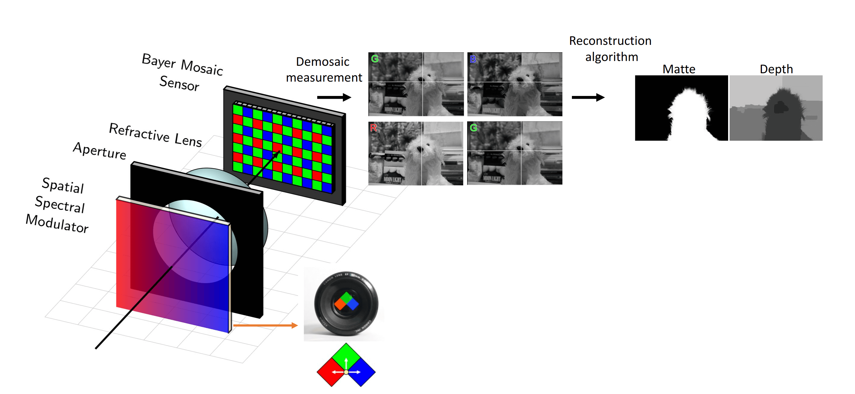
One solution to the design problem is the general architecture shown below. We classify systems that fall under this strategy as spectral multi-coded imaging systems. The basic idea is that the lens produces an image of the scene at the photosensor as usual but we now have a spatially-varying, wavelength-dependent optical mask placed at the entrance of the camera (at the aperture). This wavelength-dependent modulator serves the purpose of producing distinctly coded images on different wavelength channels. Said in another way, the modulator and the lens are paired together to result in a new lens that has a different functionality for light of different colors. Although the images carried on different wavelength channels are spatially overlapping at the photosensor plane, we can sample and measure a set of them simultaneously by utilizing a complementary mosaic of spectral filters tiled above the photosensor pixels. One common example of such filtered sensors are those with the ubiqitous Bayer RGB (red,green,blue) color filters, tiled in 2x2 arrays above the pixels as shown below. After demosaicing the measured signal, we then obtain in this case three unique images of the scene, at the cost of spatial resolution.

I emphasize that systems of this type (spectral multi-coded imaging systems) have been researched and explored in various forms for at least 20 years now! Across different tasks, the wavelength-dependent optical modulator has taken on many different forms but the general system design and functionality is exactly that outlined above. To give a concrete example, in this figure we also show the particular optical element, a set of captured images on the three channels, and the post-processed depth-map obtained from this design, as published in a work from 2008 by a research team at the University of Tokyo [3]. The wavelength-dependent optical component can thus be as simple as a spatially-varying pattern of spectral filters placed just before the lens. Three different images are carried on different wavelength bands, and they are all digitally measured using the mosaiced photosensor. By computing based on the differences of these three images, one can efficiently obtain a segmentation mask and a depth map without the need for learned priors.

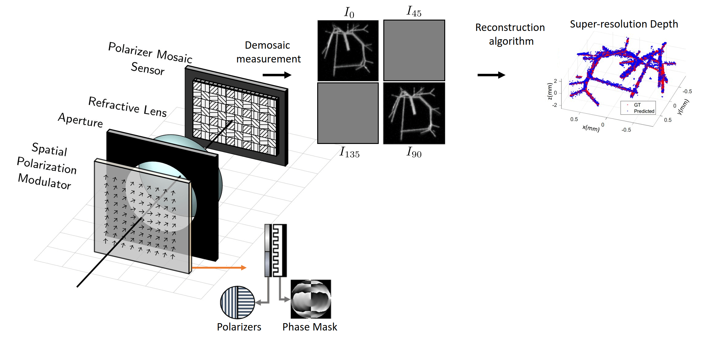
While the above systems have been extensively researched and published on, there is an alternative approach to the same task that has been largely unexplored. Rather than producing distinct codes on different wavelength channels, it is possible to instead consider producing the set of coded images on different polarization states of light. As depicted below, we only need to swap the general wavelength-dependent optical component for a polarization-dependent component, and we need to replace the array of spectral filters on the photosensor with an array of polarization filters. Fortunately, photosensors with this required mosaic of polarization filters have recently become commerciably available and widely accessible since around 2019. You can now buy these photosensors from almost every optics store just like with the RGB photosensors (see the Polarsens tech made by SONY as an example). Introducing this simple change reveals some important advantages relative to the spectral coding counterpart and in this work, I discuss a particular problem that cannot be done without switching to polarization coding. For those who are rusty or unfamiliar with the concept of polarization in light, check out Lucid Vision Labs nice summary of the concept.

Before we get into the technical details of this system, let's look at a concrete example. To the best of my knowledge, there is only one other work at the time of this publication that has considered this general design principle of using polarization to simultaneously capture multiple coded images of a scene in a single snapshot--that is the very recent work from a team at Rice University, published in 2022 [4]. Their camera configuration is slightly different but we may reduce its description for demonstration purposes to that depicted below. They utilize a diffractive phase mask to produce a two-lobe, rotating point-spread function, often called a double-helix point-spread function (if you are interested, you can see this article for more background). In addition to this element, they also introduce a polarization-dependent modulator which is simply two linear polarizers placed side-by-side--a linear polarizer orientated at 90 degrees covers the left half of the phase mask while another linear polarizer orientated at 0 degrees covers the right half. Together, the phase mask and the polarizers produce a unique effect where the two-lobes of the point-spread function are each formed from light of orthogonal polarization states. Without a polarization camera, this distinction makes no difference but with a polarizer mosaiced camera, we can use the photosensor pixels covered by 0 and 90 degree polarization filters to extract two distinct images. It is found by the authors that having these two images, instead of just one, signficantly improves the accuracy of microscopic depth sensing. Although there are four different polarization states sampled by the special photosensor, only two were used in this work and the measured signal on the others are discarded.

The goal of our paper is to delve much deeper into understanding and formally introducing this new class of computational imaging systems (polarization multi-coded imaging systems). Specifically, we aim to answer two core questions:

• The first is about the fundamental channel capacity--What is the number of distinctly coded and useful images that we can obtain by this architecture? Instead of using only two images (and thus half the pixels on our sensor), can we utilize all four for various tasks?
• Second, can we get a sense for the potential and capabilities of these systems? Moreover, how can a camera based on this architecture be designed and optimized (specifically in an end-to-end fashion)?

In the following, we present some answers to both of these questions. We then demonstrate the usage of this architecture in both experiment and simulation for a new task that we call multi-image synthesis.

Polarization Multi-Coded Imaging

In order to answer the aformetioned question about capabilities, we first need to frame it with respect to a particular choice of optics. For that, we propose designing the system utilizing a polarization-sensitive metasurface! A metasurface is a new type of optic that is made by carefully patterning a flat glass substrate with nanoscale structures. It is worth noting that although metasurfaces have been largely isolated to university research labs over the last decade, the fabrication of these components are starting to go commercial and will be widely available to consumers at some point in the coming years (see news about the company Metalenz). We choose to focus discussion on metasurfaces as the optical component because they have rapidly emerged as one of the most powerful and versatile optical tools for controlling polarization (in particular, for introducing a spatially-varying polarization transformation).

The functionality of a metasurface can be understood simply by the following: We consider a uniform grid of 350x350 nanometer cells spread across the surface of our glass substrate. In the center of each cell, we will place a single free-standing (in our case 600 nm tall) nanoscale structure. This is shown in the figure below where we use nanoscale rectangular pillars, often referred to as a nanofins. At each location, the incident light that passes through our nanostructure will experience a phase delay and by changing the shape of the structure, we can change the phase that is imparted (and to a lesser extent, the percent of light that is transmitted). Because we have the technology to independently design the shape of the nanostructure at each cell across the device, we can create a spatially-varying phase/amplitude mask that can focus light to a small point or to whatever intensity pattern we want at the photosensor. We emphasize that when the shape of the nanostructure is asymmetric like with rectangles as opposed to cubes, the optical modulation becomes polarization-dependent, which is exactly our requirement! While the discussion of nanoscale engineering deserves its own post, we may briefly note for now that there are many unique benefits to defining the modulation pattern with a sub-wavelength resolution although we wont go into details here.

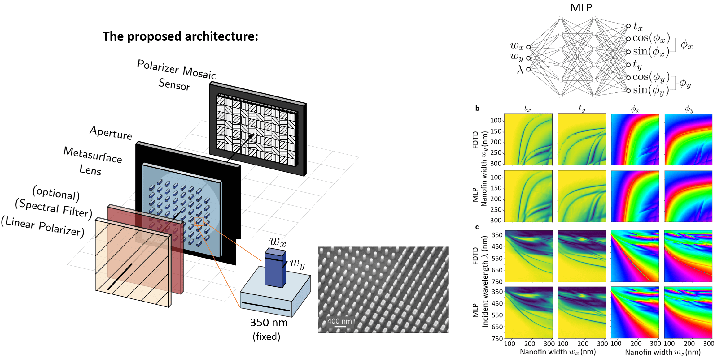
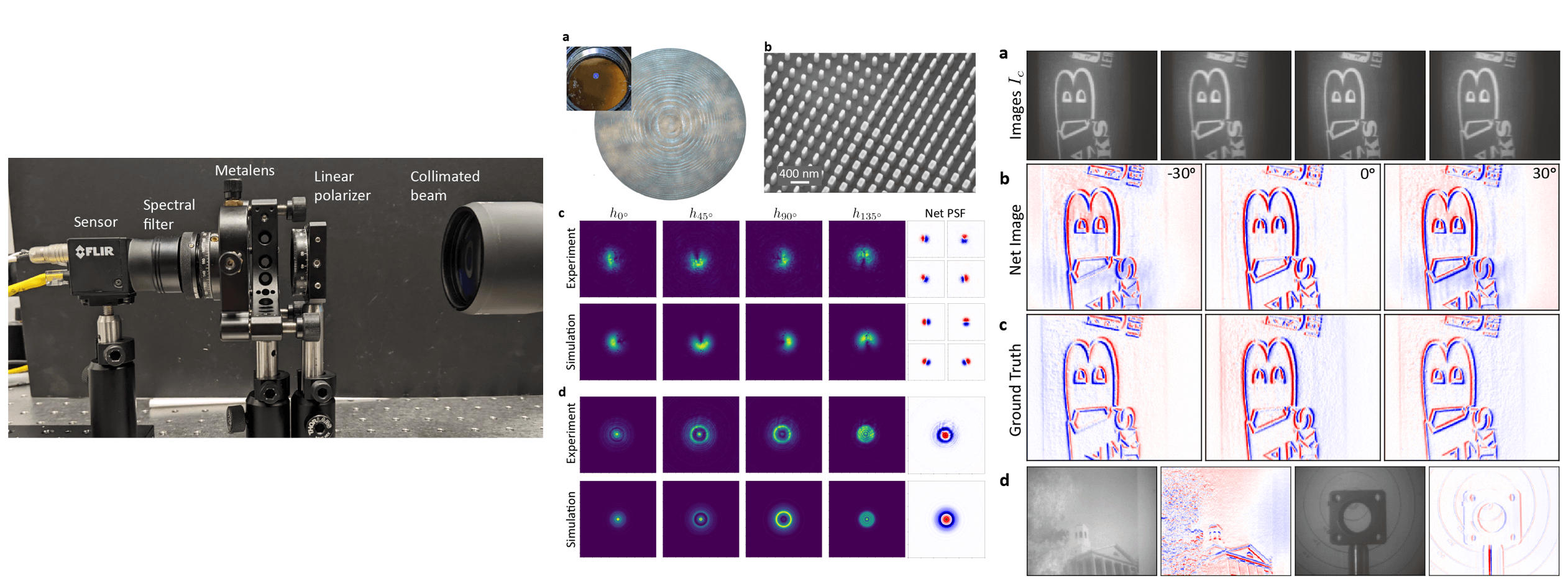
In the figure above, we depict what the general polarization multi-coded imaging system will look like when utilizing our "birefringent" metasurface. We also show a picture of a real metasurface composed of nanofins, captured using a scaning electron microscope. The metasurface here combines the role of both the focusing lens and the "spatial polarization modulator" from before and replaces the bulky optics with a single flat optic. Not only will the camera be functional, it will thus also be ultra compact and light weight. Now although we know that the shape of the nanofin controls the local transmission of light and the phase delay imparted to the incident field at each cell, how do we know the exact value of these modulations? To determine this, we actually have to directly simulate the optical response for every possible nanostructure we want to use; Specifically, we must compute solutions to Maxwell's equations for every cell instantiation to see how the field interacted with the nanostructure. Technical details are discussed in the main paper and in the supplement, but we utilize a commercial field solver and generate a dataset mapping the shape of the nanofin (its width along two directions) to the phase and transmission imparted for normally incident light of two orthogonal polarization states. We emphasize that this mapping is strongly dependent on the wavelength of the light and for this reason, the calculation must be directly evaluated for all wavelengths that we want to consider. While there are some tricks and approximations for various nanostructures that people have proposed to avoid doing these calculations, there is in general no way to accurately deduce the answer without using a field solver.

With this dataset generated, we can stitch together the response of each cell to define the functionaity of the full metasurface, and we can simulate the image(s) that would be measured by our camera for any scene. The task is then to identify a metasurface (i.e. the shape of the nanofin to be placed in every cell) which will produce a set of polarization-coded images that benefits our computational sensing task. To do this, we will run an end-to-end optimization and use gradient-descent to iteratively update the metasurface design and any learnable parameters in the reconstruction algorithm until a target loss function is minimized.

It should be emphasized that we do not want to simply learn a pair of phase masks for one or more wavelength channels, i.e. the phases \(\phi_x, \phi_y\) from above, because our metasurface cannot realize any arbitrary, user-defined transformation. Said another way, there are countless optical response that we might specify at a given location which cannot be produced using any of the nanofin shapes in our dataset. This problem is especially exasperated when we want to optimize the optic for broadband usage because our ability to produce completely different transformations for different wavelengths is quite limited. To get around this, what we want to do is optimize the set of shape parameters that describe the nanostructure at each cell and to back-propagate the gradients through the shape-to-optical-response mapping.

Motivated by the use of coordinate-MLPs in NERF [5], we train an MLP to serve as an auto-differentiable, implicit representation for the dataset. We find that just two fully connected layers with 512 neurons in each is more than sufficient to learn the representation, as shown in the right-most display in the above figure. In the paper, we also test and benchmark the use of elliptic radial basis function networks and simple multivariate polynomial functions; however, we find that the presented MLP yields substantially better accuracy with reasonable computational costs. This method also is also far more efficient than directly computing the optical response of each cell utilizing an auto-differentiable field solver and it enables us to optimize much larger lenses. Throughout, when we discuss optimizing the metasurface, it is implied that we are referring to optimizing the shape parameters for each cell by back-propagating gradients through the pre-trained MLP (whose weights have been frozen after initial training).

Polarization Channel Capacity

Before introducing one particular task that we want to solve with this system, we first raise a fundamental question about the channel capacity of this architecture. Given our polarization-sensitive metasurface and a scene that emits unpolarized light, how many of the four channels on the polarizer-mosaiced photosensor can we engineer and code? In the spectral multi-coded imaging system discussed above, the answer is unambigous. If we presume that the Red, Green, and Blue filters have transmission curves that are non-overlapping, then we can capture three distinctly coded images since different wavelengths of light do not interfere with each other. In the polarization multi-coded imaging scenario, the answer is less clear because we will have to consider the interference of our polarized light.

As a reminder, when we talk about a coded image, we mean a measurement that is formed and captured by a camera that has specialized optics that do something different than just focus all light from a point in the scene to a single pixel on the sensor. Broadly, these special cameras contain one or more carefully engineered optical modulation patterns, i.e. phase and/or transmission masks, which may possibly be paired with the usual focusing lens. Later, you will see that we are more formally referring to imaging systems that have structured point-spread functions (like the double-helix point-spread function mentioned previously), but for now, let us not worry about the exact definition of coding or this technical detail. Let us simply assert that the number of distinctly coded imaging channels accessible to us corresponds to the number of intensity patterns that we can independently design and extract when our camera is illuminated by a beam of light. This scenario is qualitatively depicted below for our polarization multi-imaging setup. For conceptual simplicity, let us approximate the polarization-sensitive metasurface as a pair of independent, idealized phase masks. Each mask has unity transmission and operates on only one of two orthogonal linear polarization states, imparting a spatially-varying phase modulation \(\phi_x\) or \(\phi_y\).

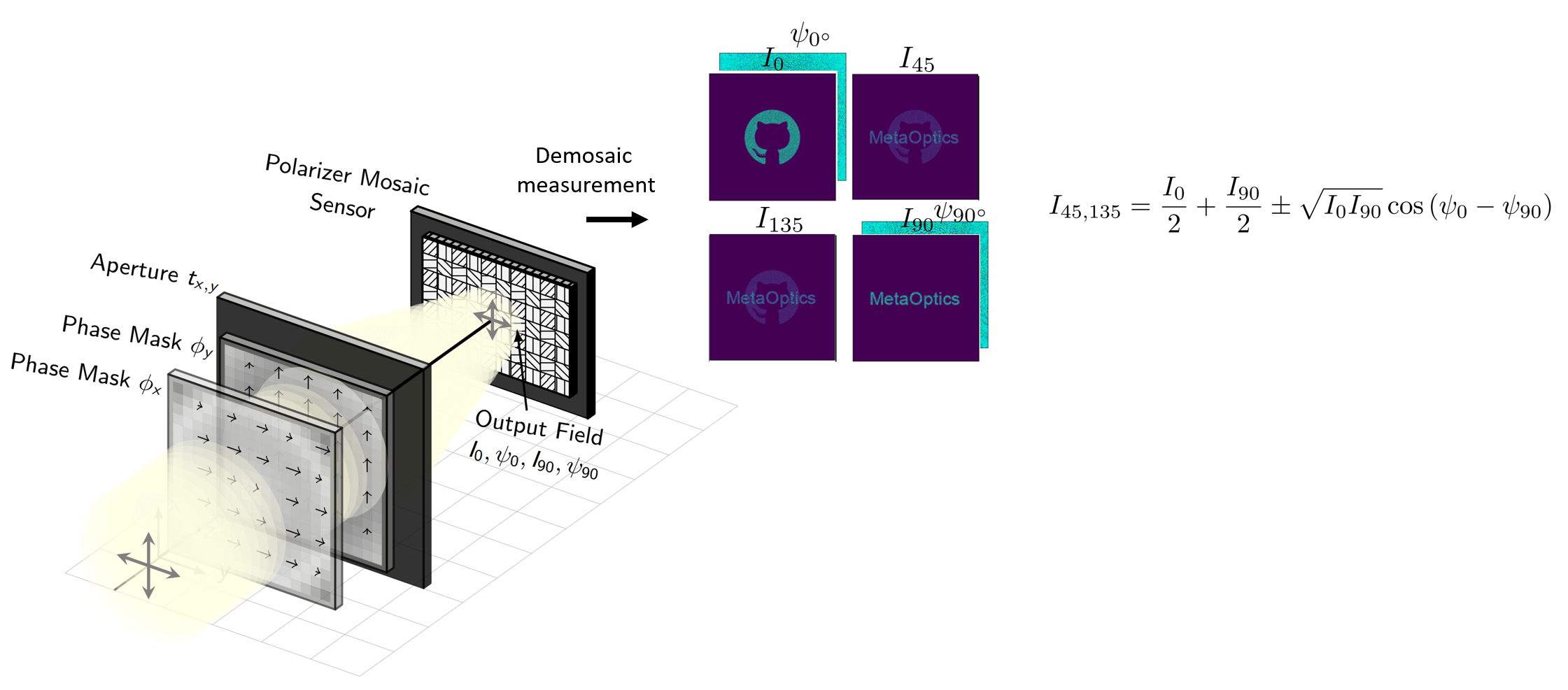
Taken in this scenario, the answer becomes clear--in a rigorous sense, this particular polarization-encoded architecture has only two channels that we can exactly control. Note that this statement is a little too strict and doesn't exactly hold if we assert that our metasurface can modulate the intensity in addition to the phase of the incident light; however, we will stick with this more constrained bound since most of our nanofin cells have similar transmittance. To see why the channel capacity here is only two, consider that we can independently control the intensity pattern that is induced and measured on the 0 and 90 degree filtered photosensor pixels (aligned with the x and y-axis of our reference frame) by independently designing the \(\phi_x\) or \(\phi_y\) phase masks patterns. Now although the photosensor can only measure the total intensity \(I\) of the light that hits each pixel, the light also has a relative phase \(\psi\) when it arrives which is also important for us to to keep track of. Given the phase and intensity of the light that arrives at the photosensor for the two polarization states, \(I_0, \psi_0\) and \(I_{90}, \psi_{90}\), the intensity that we will measure on the other two sets of filtered pixels (the pixels with \(45^\circ\) and \(135^\circ\) degree linear polarizers above them) is then fixed and defined. Specifically, we can write down this intensity in terms of the interference of the two designed channels using the equation shown in the figure above.

Thus in a rigorous sense, we state that we can only freely design the codes (and in more technical terms, the structured point-spread functions) for two of the four channels. You may be wondering if it is possible to design the intensity patterns on three of the channels, say \(I_0, I_{90}, I_{45}\), by somehow using the parameters \(\psi_0, \psi_{90}\) as degrees of freedom that can tune the interference-- notably, we don't really care about what the phase of the field is when it arrives at the photosensor, we only care about the intensity that we measure. Unfortunately the answer is no. For any polarization state, if we specify the intensity pattern of the light at two planes in space, say at the aperture where our phase masks are placed and at the photosensor, then the phase of the light everywhere is instantly fixed. In other words, specifying the intensity pattern at the sensor correspondingly specifies the phase at the sensor and so it isnt a degree of freedom at all in the traditional sense. You can rigorously prove this statement by discussing the transport of intensity equation, but we wont get into that here.

Now a key insight and motivation that we emphasize in our paper is that while the rigorous answer is that the channel capacity is two, the practical answer--which is the answer we care about--is that the channel capacity is in fact three (but with a caveat!). The underlying argument is simple, however, the amount of flexibility that it grants is rather suprising. Instead of talking about an exact intensity pattern produced at the photosensor for any one channel, let us consider the infinite number of intensity patterns we might alternatively accept that are similar to the one we wanted.

For example, if we specify a target intensity distribution \(I_{90}\) that is just a uniform circle of light at the photosensor, then there are an infinite number of phase masks that we could design to produce intensity patterns that approximate a uniform circle. Because every distinct intensity pattern at the photosensor plane \(I\) also has a distinct phase \(\psi\), we actually can specify the pattern on two orthogonal polarization states and simultaneously structure the light formed by their interference! The caveat is that we have to be okay with utilizing intensity patterns that approximate the ones we want with some amount of error. In other words, there exists a very large but constrained space of all possible tuples of intensity distributions and our design task is to learn to select from this space. As an aside, it is interesting to consider that this caveat is rather reasonable given the fact that we never had the ability to realize specified intensity pattern exactly to begin with! Finding the optics that produces a particular intensity pattern, often known as the problem of holography, is an inverse problem that can only be solved by utilizing iterative gradient-descent based methods that minimize (but never zeroes-out) the approximation error. We might not have necessarily appreciated or considered, however, that the presence of approximation errors actually increases our channel capacity when used properly.

Before we continue, let us first formally consider what may happen when we introduce/allow for errors in our intensity approximations (see the diagram below). When we compute the intensity that is induced on the photosensor by our optic, we do so over a finite domain which we refer to as the simulation region. We might try to make this calculation grid as large as possible but it will always have a finite area. Our target intensity pattern is specified explicitly over the simulation region and is it is implicitly presumed to be zero everywhere outside that domain. We then would like to learn an optic that approximates this pattern, perhaps only up to scale so we need not worry too much about normalization.

• One potential outcome after optimization is that our designed optic focuses all the inicident light into the area prescribed by the simulation region but the intensity within this region disagrees to some extent with our target.
• Another outcome is that the optic scatters some amount of this incident light to areas outside of the simulation region but it learns to match the target distribution almost exactly (up to scale) within the region.

These two cases are interesting but we have to be particularly careful to remember the implicit approximation error hidden in the second case, where light is being sent to regions that we are not directly computing the intensity on. We choose to bring attention to this detail because it has some important consequences. First, when you do not have careful accounting of the light and allow some of it to disappear (from the perspective of the calculation), then you can trick yourself about the channel capacity. In this case, you actually can make three intensity distributions exactly within the simulation region (although they of course disagree outside of it)--the previous argument doesn't work here because we have no longer specified the intensity everywhere on the two planes. There are interesting things that can happen here like super-resolution imaging, but we strongly want to avoid allowing this type of approximation error! Scattering light outside is problematic because it will produce a diffuse background that reduces the contrast of any signals in our measurements. It will break many of our algorithms and result in measurements that do not look like images of the scene at all. Importantly, without explicitly adding regularization terms that penalize this behavior to our gradient descent algorithm, attempts to optimize the intensity on three channels will immediately default to applying this strategy of scattering light outside the simulation region.

This is intuitive: if you defined the L1 or L2 loss between the target intensity patterns and the ones produced by the system within the simulation region, the minimum approximation error occurs when you use this trick to match the intensities on all three channels as close as possible. Even if you do an end-to-end loss based on images or task performance, you will still run into the same issue (hopefully you can see why). We will mention regularization again briefly at the end of this post but we leave the technical details to the main paper. The take-away is that we can sample the space of approximators but we must use additional regularization to also enforce that the light is spatially contained. Fortunately for us we find (and demonstrate below) that just using the mismatch errors within the simulation region grants enough flexibility to structure all three channels in a way that is meaningful for most imaging tasks.

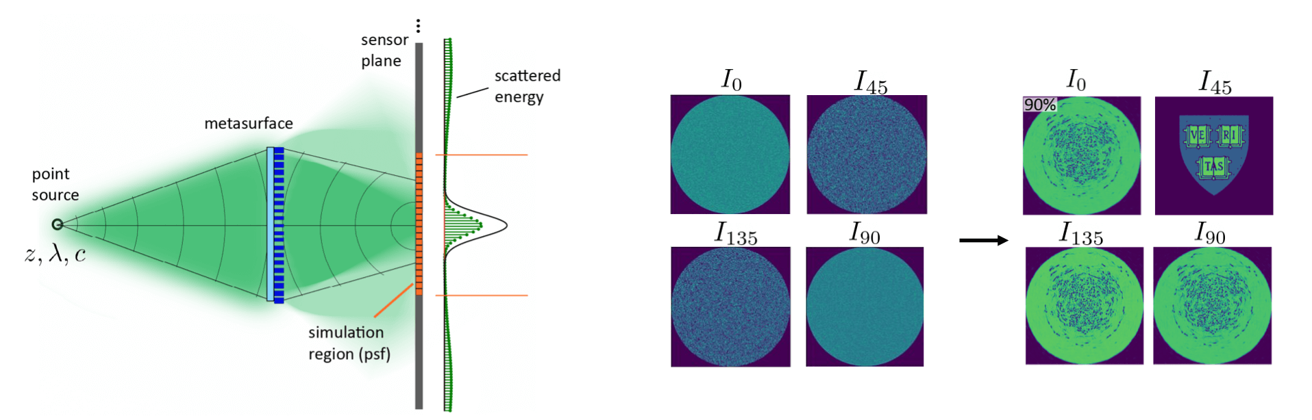
To conclude this section, we give a demonstration of these ideas tied together. First, we specify a pair of target intensity patterns (set to uniform intensity disks of light) and optimize a metasurface composed of nanofins to induce these two intensity patterns for monochromatic, linearly polarized light orientated at \(0^\circ\) and \(90^\circ\) degrees. The resulting intensities are shown above in \(I_0\) and \(I_{90}\). The pair of realized intensity distributions have low approximation error and the intensity measured on the other two channels, formed from the interference, also look like disks. Next, we keep these two target intensities but now add in a third target by specifying the target intensity on the \(45^\circ\) degree channel to be the Harvard crest. We use regularization during gradient descent to enforce that light at the photosensor plane is kept within the simulation region, and the result is shown on the right. Just by introducing some variations in our intensity approximations on the \(0^\circ\) and \(90^\circ\) polarization channels, we open up the design space on the third channel and can produce user-defined intensity patterns.

Multi-Image Synthesis Problem

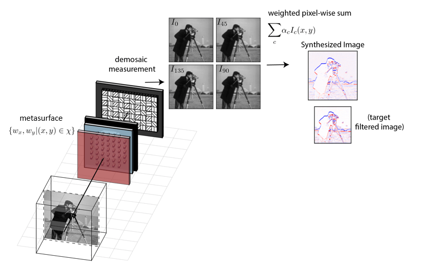
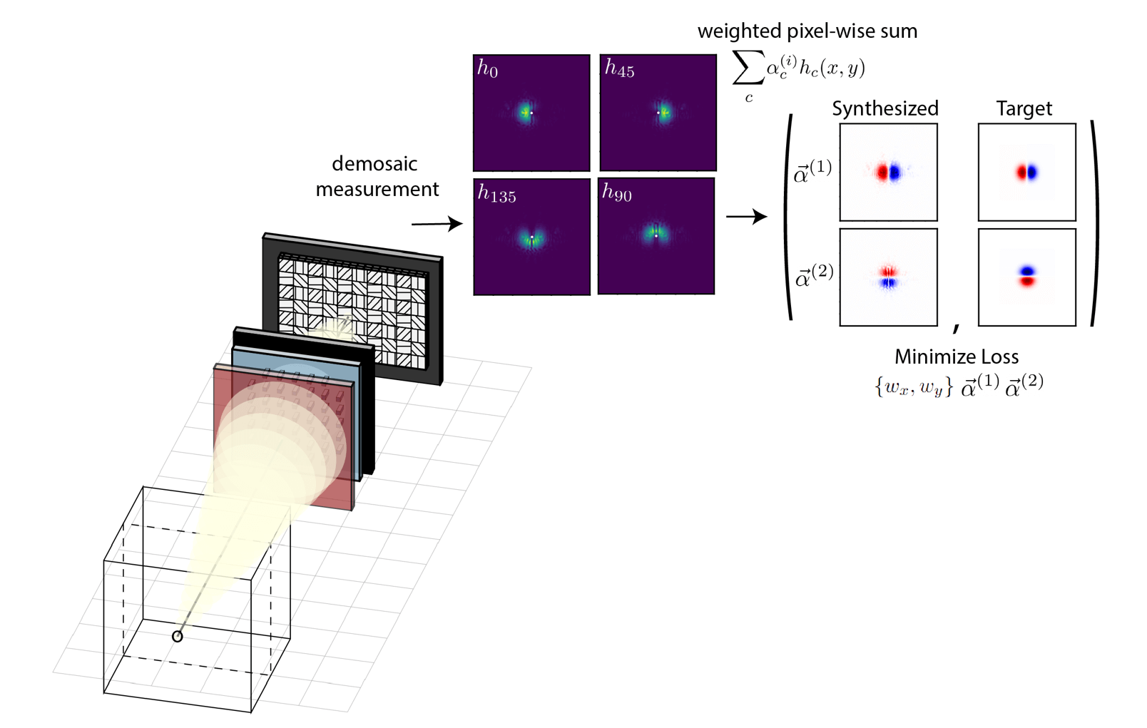
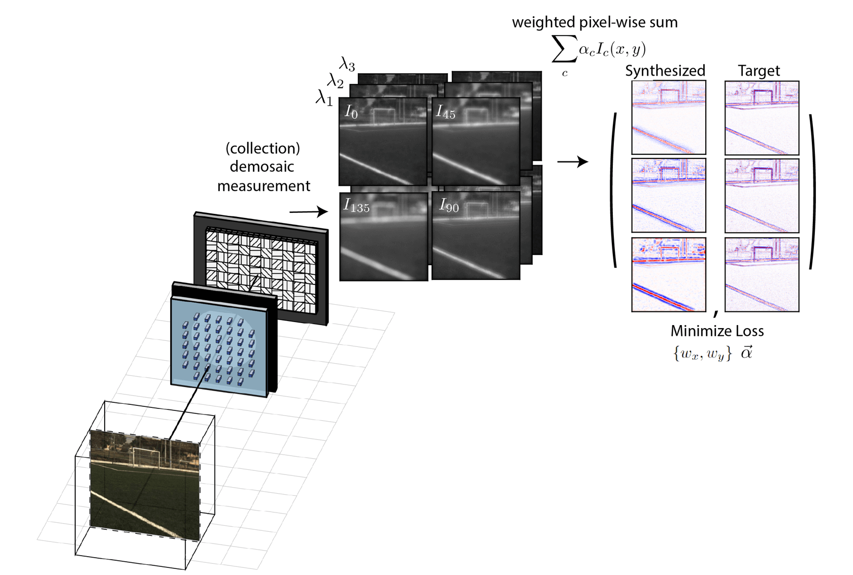
We now would like to apply this technique of polarization multi-coded imaging to a new task that we introduce in this work, referred to as multi-image synthesis. I will outline the problem here and then explain how it relates to (and is distinct from) a large body of research conducted in the 1970s on optical image processing. The task in its simplest form is depicted in the diagram below and can be stated as follows: Given a scene that emits incoherent light, we design our metasurface camera to capture a polarization-encoded measurement. This measurement is then demosaiced to obtain four distinctly coded images of the scene. By digitally computing only the pixel-wise linear sum of the four images \(\alpha_{1}I_{0}(x,y) + \alpha_{2}I_{45}(x,y) + \alpha_{3}I_{90}(x,y) + \alpha_{4}I_{135}(x,y) \) with scalar weights \(\alpha_c \), we then obtain a newly synthesized image corresponding to a spatially filtered version of the scene. By co-optimizing the metasurface and the digital synthesis weights, we can produce different filtering kernels. Moreover, through this single operation, we can also create an imager that applies different filter kernels to different regions in the synthesized image depending on the distance of objects in the scene or the color of the light! For those who are less familiar with general idea of image processing, you can check out these lecture slides for a brief review and introduction.

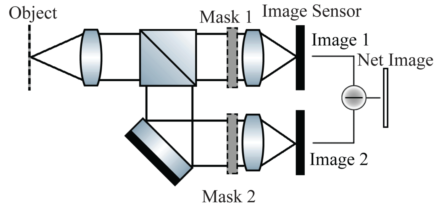
Let us briefly consider some historic motivations for this principle. It is clear that applying basic image processsing operations can be done entirely digitally, just by capturing an in-focus image and then doing a digital convolution with some filtering kernel. Half a century ago, however, computational power was far more limited and expensive than it is today. This fact spurred substantial research on optical image-processing. As an aside, if you are interested in this general topic, I would recommend the following book [6] published in 1981; although times have changed, the underlying physics has not. While it was unfortuntely proven around that time that there can be no purely optical implementation of spatial frequency filtering for scenes illuminated by incoherent light, the underlying idea of combining coded measurements with a digitaly implemented subtraction operation emerged as the next best thing. Systems were then built like that shown in the 1978 paper published by A. Lohmann and W. Rhodes [7] (Click here to see a diagram of their setup). A beam-splitter was placed inside the camera to split the light incident on the aperture into two seperate paths. Different optics (phase masks) were then placed in each path and two seperate photosensors were used to capture the pair of coded measurements. Sadly, we might note that this is a very large and specialized optical setup that can only implement a single spatial frequency filtering transformation--even if its usage saves us several million floating point operations per frame, this gain alone does not feel like much in the age of commodity Ghz processors!

×

With that in mind, my purpose in revisiting the task of opto-electronic image processing is not to simply re-argue the idea of using optics to reducing computational costs for computer vision tasks. Instead, I focus on this problem for two reasons: (1) I use it to establish the capabilities, benefits, and design principles for the newly introduced polarization multi-coded imaging architecture; and (2) we demonstrate that this method of capturing and processing on a collection of optically coded measurements can lead to new functionality and can produce synthesized images that have no simple, purely digital counterpart.

Delving deeper into the first point, I want to highlight just how compact our camera is relative to all previous designs. While in some cases we put a spectral filter at the entrance of the camera, at minimum we only have a single optical component--a very thin, flat metasurface--in addition to a single commercial photosensor. This means that the advantages and new functionality that we obtain do not come at the trade-off of camera size or weight! Moreover, this is actually the first ever single-optic demonstration of incoherent image processing that is suitable for all general scenes. This last point is a little subtle but it is important for us. Researchers in the past have tried to re-implement the original 1970's work to create a single filtering operation but with smaller optics by applying the previously discussed spectral multi-coded imaging technique [8]. This spectral paradigm however will not generally work for this task, and it highlights that there are cases where we must instead switch to the new polarization anologue.

To see why, let us emphasize that we want all four demosaiced images of the scene to be identical excluding the optical code. This is true in the polarization architecture, because if we removed the metasurface and placed a standard (polarization insensitive) focusing lens, then the images on the four channels will be the same, assuming the scene emits light that is unpolarized. If we are unsure about the scene, we can enforce our requirement by placing an additional linear polarizer at the entrance of the camera, orientated at \(45^\circ\) relative to the x-axis. Our system will then work as intended in any case. This fact is not true however for a camera designed with the spectral multi-coded imaging principle. If we place a regular lens infront of a Bayer moisaced photosensor (a mosaic of spectral filters above the pixels), we immediately know that the images captured on the different color channels will not be the same. A set of identical images require that only white light is emitted from the scene which is very unlikely. Consequently, the spectral coding case can be useful when our post-processing algorithm does not care about differences in the relative brightness between images and if semantic/spatial content is all we need. This is not true for our multi-image synthesis problem! If the intensity intrinsically varied across the set of images in a way that depends on the scenes, we cannot define a single set of constants \(\alpha\) such that the subtraction of images will always remove the correct amount of signal from various regions. In summary, the polarization multi-coded paradigm can be used for any computational imaging task while the spectral counterpart must be considered more cautiously (and cannot be used here).

Lastly, I mentioned that I will use this system to demonstrate some new optical image processing functionalities that, to the best of my knowledge, have never been previously discussed. In the following section, I show some results and explain at a high level how we run the end-to-end optimization of the camera. The three main functionalities that we looked at in this paper include the following:

• We use the snapshot measurement from a single exposure and obtain different filtered images by only changing the digital summation weights \(\alpha\).
• We specify different spatial frequency filters for different depths and obtain synthesized images that clearly encode the distance of objects in the scene.
• We introduce a method to design the spatial frequency filtering operations with respect to the wavelength of light. While it may be used to encode hyperspectral information, we use this technique to create a multi-image synthesis that can be used in a broadband setting.

Multi-Image Synthesis Optimization

Throughout this section, you will see that we optimize over and utilize all four of the images that are obtained after demosaicing the camera's measurement. You might be wondering why we use all four when the actual channel capacity is just three. When it comes to solving this particular image processing problem, there are some subtelties that motivate our choices. We mostly defer discussion of these technical details to the main paper, but this question about using three or four channels is potentially applicable for other computational imaging tasks and is thus worth commenting on. From the discussion in the previous sections, we know that we can effectively engineer the optical code applied to three of the channels, say the demosaiced signals \(I_0, I_{45}, I_{90}\). The fourth signal \(I_{135}\), although distinct, is actually not linearly independent and is equivalently given via \(I_{135} = I_0 + I_{90}-I_{45}\). In theory, we thus need not measure it because we could alway obtain it digitally. In practice, however, we should not discard it because this equivalence assumes a noiseless measurement. Consider instead a noise operator \(\Gamma()\) which corresponds to Poisson and Gaussian noise added to the signal when we try to measure it. We are then actually comparing the direct measurement of \(\Gamma(I_{135})\) vs its linear combination from noisy components \(\Gamma(I_{0}) + \Gamma(I_{90}) - \Gamma(I_{45})\). One always prefers the former and it is particularly helpful when operating under low light conditions.

(1) Multiple Filters through a Single Exposure

Previous opto-electronic image processing systems are only able to realize a single spatial frequency filtering operation in the synthesized image. The reason for this can be fully attributed to the fact that only two coded images were captured and used. In our new architecture, however, we actually have three distinct imaging channels and this simple increase allows us to encode multiple functionalities in a single snapshot. Specifically, the number of filtering operations that we can selectively apply in the synthesized image just by using different summation weights \(\alpha\) can be shown to increase non-linearly with the number of coded images that we can capture. In other words, more is really better for the task of multi-image synthesis.

To understand this further, it is useful to think about the operation of our camera in terms of the (incoherent) point-spread function. The point-spread function is the intensity pattern that is induced by the optics and measured by the photosensor in response to an ideal (in this case axial) point-source placed in front of the camera. This is visualized in the left side of the diagram below. Because every scene may be approximated as a collection of such point-sources that emit light towards the camera, specifying the point-spread function (for all wavelengths of light and all scene depths) fully prescribes the functionality of the camera. In our particular architecture, because we demosaic the measured intensity pattern to obtain four distinct images, we may say that our camera has a set of four distinct point-spread functions--one for each polarization channel. One key thing to note is that these intensity point-spread functions are purely positive signals--it wouldnt make sense if our photosensors reported negative amounts of light! For clarity, lets also refer to the point-spread functions using the variable \(h_c\) for \(c \in \{0, 45, 90, 135\}\) and reserve the variables \(I_c\) for the retrieved, demosaiced images taken of the scenes.

Creating optics that can realize certain spatial frequency filtering operations in the linearly synthesized image can now be fully understood as a task of point-spread function engineering. The mathematical formulation is noted in the paper but a key idea is that the measurement produced by our camera on each polarization channel may be approximated as an all-in focus image of the scene that is convolved with the per-channel point-spread functions. When we take the digital, linear sum of the four images, we get a newly synthesized image that corresponds to convolution with an effective, synthesized point-spread function \(\sum_c \alpha_c h_c(x,y).\) That is the heart of the particular inverse problem we want to solve! If a user specifies a particular filtering kernel, we need to find a set of digital weights paired with a set of positive point-spread functions produced by a metasurface that can be linearly combined to approximate the kernel. The optics will then do the convolution for free. This whole process is outlined schematically below.

In a more formal sense, this problem is a physics-constrained version of non-negative matrix factorization. The digital filtering kernels that we want to m ake have positive and negative values, and we need to identify a decomposition of that matrix into a set of scalar weights and positive-only signals. I want to highlight briefly that there are an infinitely many solutions to this factorization problem, but not all are equally useful when we again consider the presence of measurement noise. Trying to find the "good" factorizations from all the possibilities is one of the challenges that this paper also solves. We discuss in great length how to do this in the main paper but for this post, we will ignore these details all together. Just note that when we refer to the optimization procedure, there is regularizations applied during gradient descent to encourage favorable factorizations, in addition to the aformentioned regularization term to encourage light to be contained in our simulation region.

With these points in mind, let us now return to the comment about multi-functionality. To implement a single spatial frequency filtering operation, we need at least two channels--one channel to encode the negative signal in the target filter and another channel to encode the positive. If we have four channels, then it is quite clear that we are garunteed that we can implement two filtering operations opto-electronically. We could just use disjoint pairs of distinctly coded images and have one set of weights like \(\alpha^{(1)} = [1, 0, -1, 0]\) that implements one target filter and another set of synthesis weights \(\alpha^{(2)} = [0, 1, 0, -1]\) for the other. What is less obvious is that you can do better than this because you can reuse coded images for different tasks. In otherwords, the set of weight vectors do not need to be orthogonal which actually means that the number of operations we can implement scales non-linearly with the channel capacity! We use this fact to our advantage in this work and although we only have three channels that we can directly engineer the point-spread function on, we simultaneously implement many different filter pairs (one of which is shown here and in the main paper).

Being able to implement two filters instead of just one is exciting because of a technique in computer vision known as steerable filtering (see the article written by W. Freeman on the topic [9]). The underlying idea is that certain filtering kernels have a nice mathematical property in that they serve as basis functions for a much larger space of useful filters. Said in more technical terms, if you can create two filters, then you can also create any other filter that lies in the linear span of those two. As a concrete example, consider as the targets a pair of Gaussian derivative kernels, with one orientated along the x and the other along the y-axis. This is shown in the right-side of the above image, labelled as "Targets". If we can find a pair of weight vectors \(\alpha^{(1)}, \alpha^{(2)}\) that synthesizes these two filters from our set of point-spread functions, then we are garunteed that there is a weight vector that will synthesize the Gaussian derivative along any other angle. That weight vector would be derived via \(\cos(\theta)\alpha^{(1)} + \sin(\theta)\alpha^{(2)}\). Our optimized camera could then be used to get the derivative of the scene not just along two directions but along any direction--it implements an infinite but compact set of spatial filtering operations at the theoretically minimum computational cost. If we had access to more than three images, then we could even create other types of filter banks.

The way that we can optimize for multiple filters at once is straight forward (ignoring the various details of regularization). We implement all the calculations with auto-differentiable code in Tensorflow/Pytorch and we compute the set of four point-spread functions induced by the particular metasurface and measured by the photosensor. We then compute the linear sum of these point-spread functions using each set of synthesis weights and compare the resulting output to each of the targets kernels. The sum of the absolute value of differences (the L1 loss) is then evaluated and we may then use auto-differentiation to obtain the gradients of the loss with respect to the metasurface shape parameters--the nanofin widths \(\{w_x, w_y\}\) at each cell across the metasurface--and the synthesis weights--\(\alpha^{(1)}, \alpha^{(2)}\). Iteratively, the gradients are used to update our optics and our post-processing algorithm until the loss is minimized! Some results from this optimization is shown in the figure below:

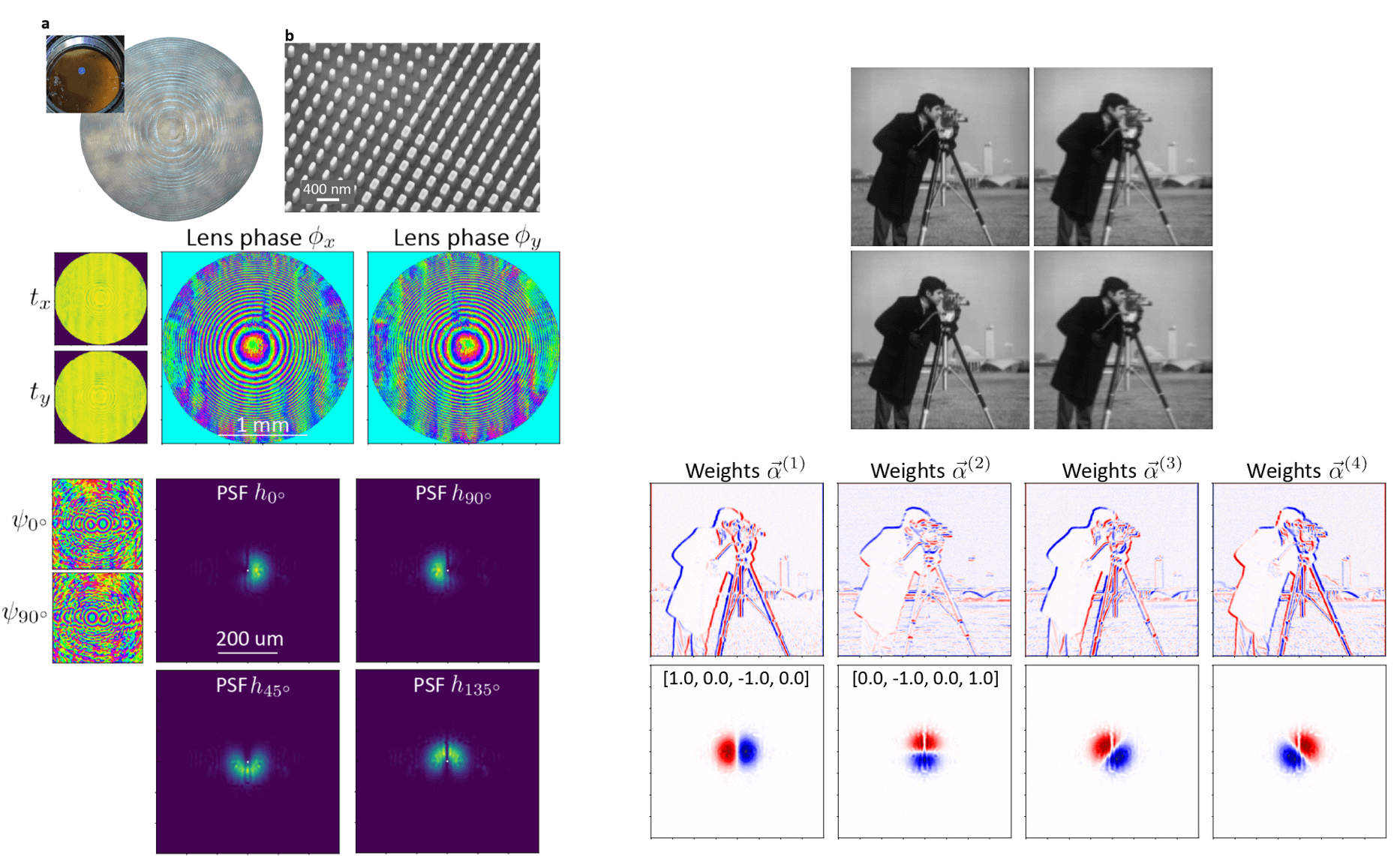
We optimize a 2 millimeter diameter metasurface (comprised of about 10+ million total parameters) which imparts near unity transmittance but different phase profiles for x and y-linearly polarized light. The set of four point-spread functions measured on the four polarization channels sampled by the polarizer-mosaiced photosensor is also displayed and clearly corresponds to a learned decompositon of the Gaussian derivative kernels. On the right hand side, we show in simulation an example of the four measured images that we would obtain when using this system. For the camera-man scene, each captured image is subtelty coded. When we compute only the linear, pixel-wise sum of the four images using the optimized scalar weights, we then obtain the first-derivative of the scene, applied at any orientation that we specify.

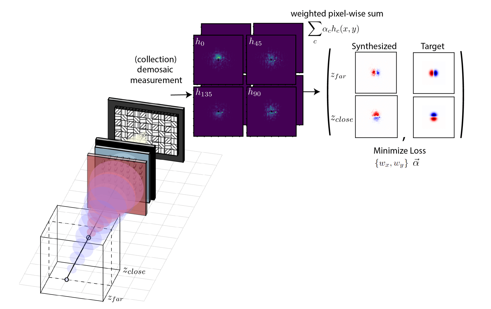
(2) Depth-Dependent Spatial Freqency Filtering

Similar to the previous example, we can also optimize the point-spread function in order to synthesize different spatial frequency filtering operations for different depths. Notably, this type of filtering operation cannot be done purely digitally without first already having an in-focus image of the scene, a segmentation mask, and the depth map. Alternatively, our optics can provide for us this type of transformation for almost no computation.

To optimize a system like this, we compute the four point-spread functions in response to a point-source placed at different distances, as shown in the figure below. For visualization, we depict just two distances but in practice, we define as many depth planes as possible. We consider only a single set of synthesis weights \(\alpha\), in contrast to the previous section, and for each depth, we specify a different target filtering kernel that we want to realize. We then compute the synthesized point-spread function for each depth and compare it to the target. The L1 loss is again used and we evaluate the sum of the absolute differences for all cases. In the paper, we look at the task of producing a Gaussian derivative filter that rotates in angle with respect to depth.

We show some results for this optimization below. As a note, we only really use two of the four channels for this task because the regularized gradient-descent (correctly) finds that a two-signal decomposition is the best factorization when one considers measurement noise. Regardless, the learned optics encodes the two halves of the Gaussian derivative kernel on orthogonal polarization states of light. Moreover, the synthesized filter rotates from 0 to 90 degrees in orientation as the point-source gets further away. Now, I want to briefly emphasize that there already exists analytic relations to define a phase mask that produces a rotating point-spread function--these are based on something known as Gauss-Laguerre modes; the metasurface that we have learned, however, does not implement that phase profile! Instead, our metasurface learns a new solution, starting from a random initialization, to synthesize rotating point-spread functions with light split on different polarization states.

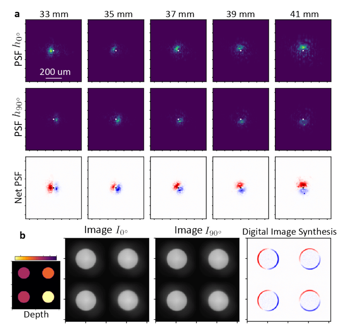
In the bottom panel of this figure, we show in simulation an example of what the synthesized image would look like when we have a scene with objects at different depths. Specifically, we consider the simple case of fronto-parallel disks of uniform intensity placed at four different distances in front of the camera (shown on the bottom left panel). The images simultaneously captured on the two polarization channels are displayed alongside the synthesized image obtained from just a pixel-wise subtraction of the two images. Interestingly, we obtain a differentiated version of the scene, but one where different spatial frequency filters have been applied to different parts of the image! Depending on the depth, the first-derivative has been taken at different angles. We propose that a system like this can be particularly effective for low-computation depth sensing. Depth is no longer encoded in the optical defocus but is instead encoded in the orientation of the derivative which is visually easier to identify. Keep in mind that we obtain these sparse depth cues alongside and co-aligned with the original undifferentiated images of the scene!

(3) Filtering with a Prescribed Wavelength Dependence

Lastly, we now discuss the idea that we can design the image filters applied by our optical system with respect to wavelength. Using the exact method introduced in the last section, we could simply specify different target filters for different wavelength values and run the optimization. The result would also be interesting in that the synthesized image would have different spatial frequency filters applied to different regions depending on the spectral content of the scene. Again, producing an image like this purely digitally would be challenging as it would require obtaining a segmentation mask and a hyperspectral measurement of the scene first.

Although we tested an optimization algorithm analogous to that in the last section based on computing the loss between the synthesized point-spread functions and the target filters, we found that it is not the most effective approach. The primary reason is that it is very easy to specify a set of target filters that are impossible for our system to synthesize. If this happens, gradient descent will not converge to something useful. Moreover, part of the challenge is also that it is not easy to know beforehand what target filters are possible or to identify similar but valid alternatives. For these reasons, we also introduce in the paper an optimization scheme based instead on rendered images which circumnavigates all these problems.

Before we continue, let us first review and explain how we can even control the behavior of our lens with respect to incident wavelength. In an earlier section, we showed the computed optical response for different nanofin shapes (click here to see that figure again). We noted that the phase and transmittance imparted by a given nanostructure will change significantly with respect to wavelength and that this wavelength dependence is different for every nanostructure. This simple fact is the key to the design task. If we want a metasurface that imparts a different phase profile to different wavelengths (and thus produces different point spread functions), we then need to choose a suitable nanostructure at each location that has the specified wavelength-dependent phase. Looking again at the figure and the optical responses that we have access to with nanofins, however, we are clearly constrained in that we cannot make anything we want. This constraint is actually quite severe and so more often then not, we will have to learn to settle for synthesized filters that are similar to but not exactly the one we specified. Things will be easier if we use more complicated nanostructures instead of the simple nanofin but we leave that for future work.

Now we would like to demonstrate these ideas with a more concrete example. In doing so, it is instructive to slightly reformulate our problem. Instead of requesting different filters for different wavelengths, let us just consider the task of producing the same filtering operation across a large wavelength range. We do this because a wavelength invariant filter is probably the simplest target operation that we know straightaway is fundamentally impossible to achieve! To be clear, it is impossible because both the metasurface modulation and field propagation (from the metasurface to the photosensor) are wavelength-dependent transformations. None-the-less, for our imaging system, we would like to target a fixed width Laplacian of Gaussian filtering kernel for many wavelengths between 500 and 600 nm.

The important insight is this: we do not want to try to learn a multi-image synthesis system that realizes this transformation exactly for all wavelengths; instead, we want only to learn a set of synthesized filtering operations that approximate the statistics of the requested Laplacian of Gaussian kernel. Consider that there are countless filters that are mathematically different from a Laplacian of Gaussian but ultimately produce a similar visual or semantic effect. In this particular case, that effect is edge-detection. In practice, we might be satisfied to settle with any of these nearby transformations (including a Laplacian of Gaussian with a different width than that explicitly specified) and that is exactly what our optimization algorithm does. The scheme is depicted in the figure below and is summarized following.

×

To optimize the metasurface and the digital weights, we first start with a hyperspectral image to serve as our scene radiance. In the paper, we show that you only need a single hyperspectral datacube for training and moreover, it doesn't need to be from a real dataset. In fact, we used a synthetic scene consisting of the camera-man image emitting the same brightness across all wavelengths in the optimization range. Notably, there are benefits to using real scene data for training but we will comment on that later. For visualization purposes, in the above schematic we show a scene consisting of real hyperspectral data obtained from the Arad1K dataset [10], displayed in its RGB projection. At each training step, we first compute the four per-channel point-spread functions for each wavelength These point-spread functions are then used with the scene radiance data to render the set of four images that would be measured for each wavelength individually. Using the digital weights \(\alpha\), we finally compute the set of synthesized images by taking the weighted, pixel-wise sum of the four rendered images. These synthesized images are compared against the target images which were obtained by convolving the scene radiances with the target filtering kernels. We then minimize the loss using regularized gradient descent to update the optics and the digital weights until the synthesized images at each wavelength approximately the target images as closely as possible.

Some results from the optimization are shown in the left half of the figure below. The top-most panel displays the synthetic scene alongside the desired filtered image that we want for each wavelength (in this case it is the same filtering kernel applied across the spectrum). After optimization, the camera succesfully learns to produce a set of four point-spread functions that can be linearly combined to approximate the target filtering kernel (see panels a-b). The synthesized point-spread function is wavelength dependent as we expect, and although its shape does not exactly match a Laplacian of Gaussian, it produces a similar type of effect (panel d). As a note, the PSNR=10 label is referring to the peak signal-to-noise ratio characterizing the captured measurement. Opto-electronic filtering has historically struggled to work in the presence of measurement noise but we also showed in this paper that using regularization during optimization can help us to find solutions that operate well even at relatively high noise levels. Here, the peak signal in the image is only ten times larger than the noise.

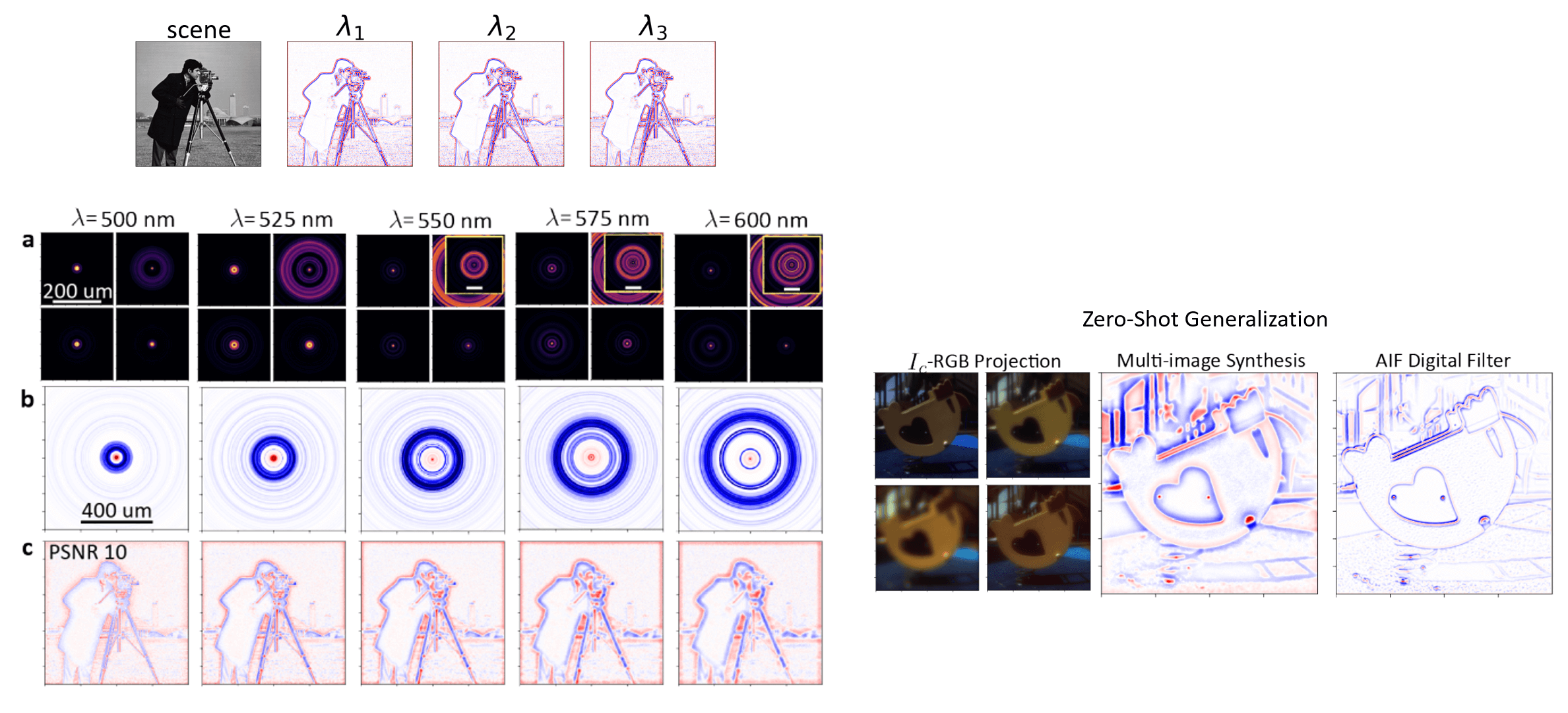
As alluded to before, we can train on a single scene because our camera is learning how to implement an image processing operation--that is, it is a mathematical transformation whose definition is independent to the input. The only requirement is that the scene utilized for training contains a diverse range of spatial frequency features. This is because we cannot learn how to filter signals of frequencies that were never there in the training image to begin with. To highlight this idea, on the right, we show the operation of the trained camera applied to a real hyperspectral image which it has not seen previously. The performance of this camera when imaging the real world, however, can be substantially improved if we used for training the real hyperspectral dataset instead of our single, synthetic scene. This would then change two things about the leearned transformation: (1) Natural scenes do not emit light equally at all wavelengths. The visual quality is more affected by errors on one wavelength vs on another and so we should have our system learn the spectral statistics of natural scenes. (2) Real world scenes have a diverse distribution of spatial frequency features. In this toy problem, the camera has learned to overfit and to prioritize filtering only the frequency features that it saw in the cameraman image. We need to use a diverse range of images during training to avoid this.

(4) Experimental Validation

Lastly, we highlight that although most of this paper was conducted in simulation to grant us the flexibility to explore different problems and to test the performance against different SNR conditions, we also built a prototype camera and captured measurements. Some of the results are shown below:

Future Outlook: Polarization + Spectral Multi-Coded Imaging

Lastly, I want to conclude this post by highlighting what I think might be one possible future for this general paradigm of multi-coded imaging. In the introduction section, we made the observation that a large of body of research in computational imaging could be grouped and classified as spectral multi-coded imaging systems. We then introduced an alternative and new paradigm called polarization multi-coded imaging. Although discussed in this paper as a disjoint architecture, I now highlight that the two design methodologies may be merged together (i.e. spectral-polarimetric multi-coded imaging systems)! Specifically, at the photosensor we can consider a combined mosaic of spectral and polarization filters placed above the pixels as shown below. The obvious trade-off here is the loss of spatial resolution but keep in mind that measurements obtained from this system will be used in post-processing algorithms. Neural networks trained on the right data are extremely good at upsampling and fixing this resolution problem. In this case, we could use spatial-polarimetric-spectral statistics to learn to restore full resolution images.

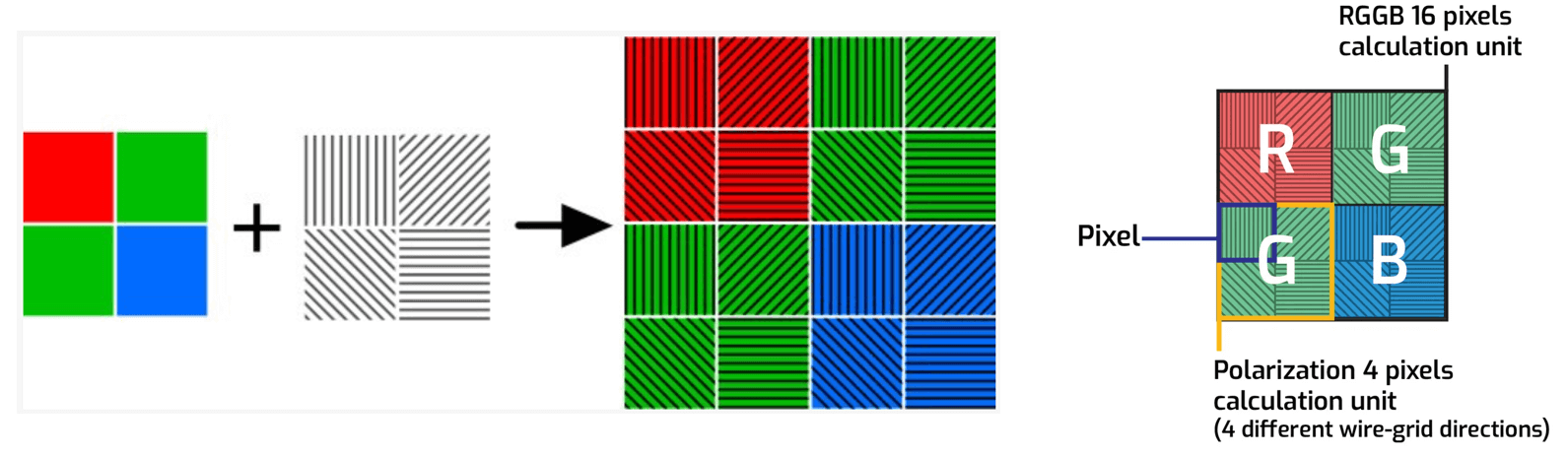
The actual camera would otherwise look the same with just a metasurface optic placed in front of this mosaiced photosensor. Again, metasurfaces may be one of the best optics to use in the design of this system because it allows the user to engineer both a wavelength-dependent and polarization-dependent optical response with a sub-wavelength resolution! In this case, instead of four images, 16 distinctly coded images can be captured in a single snapshot and used for post-processing. Moreover, if we also adapt another imaging technique introduced in [11] where a metasurface produces different images on different halves of the photosensor, this number would double to 32. It is thus theoretically possible to capture 32 distinctly coded images in a single snapshot, using nothing more than a single flat optic metasurface and a single commercial photosensor. What to do with these images will be left for future imaging and vision scientists but as noted in the motivation section, every task can benefit from processing a collection of images.

References

1. Takashi Nagata et al. ,Depth Perception from Image Defocus in a Jumping Spider.Science335,469-471(2012)
2. A. P. Pentland, "A New Sense for Depth of Field," in IEEE Transactions on Pattern Analysis and Machine Intelligence, vol. PAMI-9, no. 4, pp. 523-531, July 1987
3. Y. Bando et al., Extracting Depth and Matte using a Color-Filtered Aperture, ACM Trans. Graph. 2008.
4. B. Ghanekar et al., “Ps2 f: Polarized spiral point spread function for single-shot 3d sensing,” ICCP 2022​
5. https://bmild.github.io/fourfeat/
6. Casasent, David & Lee, S. H. (Sing H.), 1939-. (1981). Optical information processing : fundamentals / edited by S.H. Lee ; with contributions by D.P. Casasent ... [et al.]. Berlin ; New York : Springer-Verlag
7. Lohmann AW, Rhodes WT. Two-pupil synthesis of optical transfer functions. Appl Opt. 1978 Apr 1;17(7):1141-51.
8. Haiwen Wang, Cheng Guo, Zhexin Zhao, and Shanhui Fan, ACS Photonics 2020 7 (2), 338-343
9. Freeman, W. T. & Adelson, E. H. (1991). "The design and use of steerable filters" (PDF). IEEE Transactions on Pattern Analysis and Machine Intelligence. 13 (9): 891–906.
10. B. Arad et al., “Ntire 2022 spectral recovery challenge and data set,” in 2022 IEEE/CVF Conference on Computer Vision and Pattern Recognition Workshops (CVPRW), 2022, pp. 862–880
11. Qi Guo, Zhujun Shi, Yao-Wei Huang, Emma Alexander, Cheng-Wei Qiu, Federico Capasso, Todd Zickler. "Compact single-shot metalens depth sensors inspired by eyes of jumping spiders." Proceedings of the National Academy of Sciences (PNAS), 2019.